Ph-el + ph-ph Transport Tutorial
Overview
While in many semiconducting and insulating systems phonon transport is dominated by phonon-phonon scattering, in metals and some systems at low temperature, it’s necessary to include both the phonon-phonon and phonon-electron scattering in the calculation of lattice thermal conductivity. Additionally, in metallic systems the electronic part of the thermal conductivity often provides the largest contribution to the thermal conductivity. Because Phoebe offers both electron-phonon and phonon-phonon interactions, we can calculate the full thermal conductivity \(\kappa\) of a metal using phonon-phonon and phonon-electron scattering for \(\kappa_{ph}\) as well as electron-phonon scattering to calculate \(\kappa_{e}\). This is no small task, as the calculation requires the input files from both the phonon-phonon and electron-phonon calculations, and the calculation of multiple scattering rates.
Step 0: Preparing the input files
Before starting, we ask that you follow the tutorials for Phonon Transport Tutorial (steps 1-3) and Electron Wannier Transport Tutorial (steps 1-7), using the input files here for copper, stored in phoebe/example/Cu/, under the 1.el-ph and 2.ph-ph directories
(making sure to use the same crystal structure in both el and ph file generation!)
While we note that these tutorial files will result in unconverged calculations, they will serve the purpose of this example. Both sets of calculations need to be converged as described in their respective tutorials for production.
As mentioned, these can be generated by running the files in the 1.el-ph and 2.ph-ph directories. Here, * = cu and we use 3rd order force constants from phono3py.
For electrons: |
For phonons: |
|---|---|
|
|
Note
These calculations take a bit to run even though they are not production quality – ideally you will have access to more than a laptop to perform this tutorial.
Step 1: Electronic Thermal Conductivity Calculation
First, we do the straightforward step – we need to calculate \(\kappa_{e}\). This can be done as in the Step 8: Electronic Transport from Wannier interpolation step of the electron Wannier transport tutorial. All of the variables we will use are described in that tutorial, so be sure to look over what is written there.
Then, run the following Phoebe input file, which can be found in examples/Cu/3.transport/electronTransport.in:
appName = "electronWannierTransport"
phFC2FileName = "cu.fc"
sumRuleFC2 = "crystal"
electronH0Name = "cu_tb.dat",
elphFileName = "cu.phoebe.elph.hdf5"

kMesh = [20,20,20]
temperatures = [10.,25.,50.,100.,200.,300.,400.]
chemicalPotentials = [13.86829112]

smearingMethod = "adaptiveGaussian"
windowType = "population"

useSymmetries = true
scatteringMatrixInMemory = false
Here, we do a calculation across a few temperatures, and therefore, for the sake of doing a quick calculation, we use the RTA transport method. This means we don’t need to store the full scattering matrix in memory and we can run them all together to save time. In a production quality calculation, it would also be important to be sure each temperature is converged for the selected k-point mesh, as lower temperatuers will require more k-points to converge.
This should be run just as in the other tutorial:
export OMP_NUM_THREADS=4
/path/to/phoebe/build/phoebe -in electronTransport.in > electronTransport.out
Step 2: Lattice Thermal Conducivity Calculation
Now, we have to calculate the lattice thermal conductivity using both phonon-electron and phonon-phonon scattering. This corresponds to Step 4: Calculate Lattice Thermal Conductivity, step 4 of the phonon transport tutorial, but now also uses electron-phonon information.
For this, we run a Phoebe calculation using the below input file, which can be found in examples/Cu/3.transport/phononTransport.in:
appName = "phononTransport"

# specify harmonic phonon file
sumRuleFC2 = "crystal"
# must use fc2.hdf5 for phono3py,
#but could also supply cu.fc from QE for ShengBTE ph-ph
phFC2FileName = "fc2.hdf5"

# specify the paths to phonon-phonon input
phFC3FileName = "fc3.hdf5"
phonopyDispFileName = "phono3py_disp.yaml"
# supply phonon band structure information
windowType = "population"  # this will apply to the phonon states
qMesh = [15,15,15]

# path to electron-phonon coupling inputs
electronH0Name = "cu_tb.dat",
elphFileName = "cu.phoebe.elph.hdf5"
# sampling of electronic states -- will be filtered for a
# +/- max(omega_ph) window around mu
kMesh = [75,75,75]

# generic information for the calculation
temperatures = [10.,25.,50.,100.,200.,300.,400.]
chemicalPotentials = [13.86829112]
smearingMethod = "adaptiveGaussian"
useSymmetries = true
scatteringMatrixInMemory = false
Again, this should be run just as in the other tutorial:
export OMP_NUM_THREADS=4
/path/to/phoebe/build/phoebe -in phononTransport.in > phononTransport.out
Additionally, if you only wanted to run the ph-el lifetimes, there is the phononElectronLifetimes app, which can be run using an input file like the one below, found in examples/Cu/3.transport/lifetimes.in:
appName = "phononElectronLifetimes"

phFC2FileName = "cu.fc"
sumRuleFC2 = "simple"

electronH0Name = "cu_tb.dat",
elphFileName = "cu.phoebe.elph.hdf5"

kMesh = [75,75,75]
qMesh = [15,15,15]
chemicalPotentials = [13.86829112]
temperatures = [15.]

useSymmetries = true
windowType = "population"
smearingMethod = "adaptiveGaussian"
Output and Post-Processing
Below, we show the output for a well-converged version of this copper demonstration. These calculations are done with 40x40x40 q-meshes, and 400x400x400 k-meshes. It’s important to note that you should converge a calculation with respect to both – at low temperatures, you’ll be sampling a very narrow window around the Fermi energy, and therefore may need to use very dense k-meshes. This is alleviated by useSymmetries = true and an accordingly narrow electronic population window, which is used by default in Phoebe during this calculation. If symmetries are on, sometimes this requires additional sampling to reach convergence, however, there is still generally a large cost benefit to using symmetries.
Note
In these calculations, it’s important to inspect the convergence of the ph-el scattering lifetimes and overall thermal conductivity with respect to k-mesh! You may need a denser sampling that you expect.
First, we can use scripts/tau.py to plot the output ph-el, ph-ph and their combined phonon lifetimes using Matthiessen’s rule, which are stored respectively in the files, rta_phel_relaxation_times.json, rta_phph_relaxation_times.json, and rta_ph_relaxation_times.json.
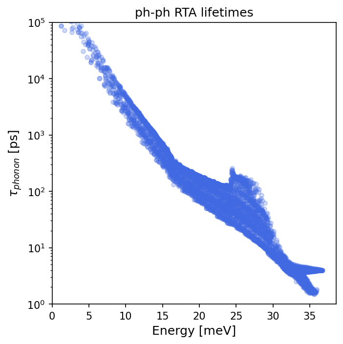
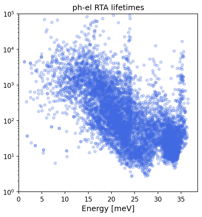
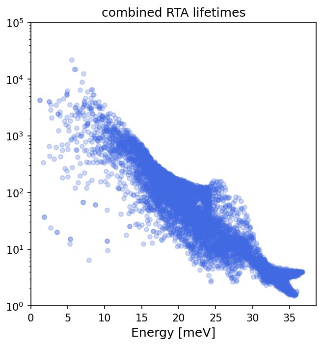
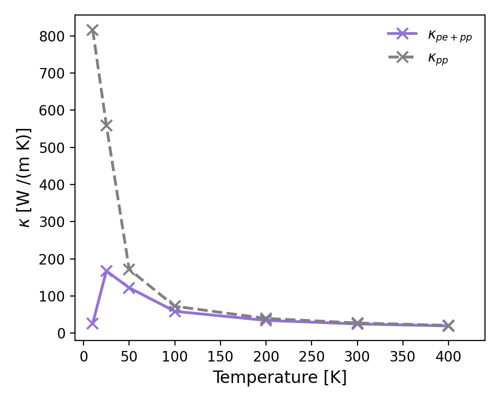
These are the lifetimes corresponding to the lowest temperature point at 10K, where we expect the ph-el scattering will have an impact on the overall lifetimes. From this, we are able to see that they do bring down the total \(\tau_{ph}\) values.
We can also inspect the effect on the lattice thermal conductivity as a result of the ph-el calculation. Here, I’ve run the calculation twice – once with both ph-el scattering, and once withe the elphFileName and other electronic parameters commented out, to run a ph-ph only calculation. From the result of this, we can see that at lower temperatures in particular, the phonon-electron lifetimes play an important role in the thermal conductivity.