Basic Band Structure and DoS
Overview
In addition to transport and lifetime calculations, Phoebe can also perform basic band structure and density of states calculations. These can be useful when debugging a calculation or checking the quality of a Wannier or Fourier interpolation. The quality of interpolation is often dependent on the number of k or q points used in DFT, so sometimes it can be helpful to run this calculation to ensure that your DFT calculation used a dense enough mesh.
Step 1: Generate input files
For this short tutorial, we’re going to use Quantum Espresso output files for electrons, and phono3py output for phonons, as generated from one of the other tutorials.
Before performing this calculation, you should either run steps 1-3 of the Electron Wannier Transport Tutorial or steps 1-3 of the Phonon Transport Tutorial. The input files necessary for the electron and phonon bands calculations are:
Electron Wannier input files
si_tb.dat
Electron Fourier input files
silicon.xml
Phonon input files (Quantum Espresso)
silicon.fc
Phonon input files (phono3py)
fc2.hdf5
phono3py_disp.yaml (or phonopy_disp.yaml harmonic only)
disp_fc3.yaml (or disp.yaml if harmonic only)
After running at least the necessary steps of these prior calculations and copying this output into your current directory (or at least, noting the path to the files so that you can specify it in the below input files), we can proceed to the next step.
Step 2: Using Phoebe to calculate band structure
Once we have the necessary input files, we run Phoebe using one of the input files below, which are also available in either example/Silicon_el/electronWannierBands.in, example/Silicon_epa/electronFourierBands.in or example/Silicon_ph/phononBands.in.
Electron Wannier bands input file
appName = "electronWannierBands"
electronH0Name = "si_tb.dat"
deltaPath = 0.1
useSymmetries = true

begin point path
L 0.50000  0.50000 0.5000 G 0.00000  0.00000 0.0000
G 0.00000  0.00000 0.0000 X 0.50000  0.00000 0.5000
X 0.50000 -0.50000 0.0000 K 0.37500 -0.37500 0.0000
K 0.37500 -0.37500 0.0000 G 0.00000  0.00000 0.0000
end point path

begin crystal
Si 0.000000000   0.000000000   0.000000000
Si 1.349401887   1.349401887   1.349401887
end crystal
Electron Fourier bands input file
appName = "electronFourierBands"
# note that this XML file should be from an NSCF run
electronH0Name = "silicon.xml"
deltaPath = 0.1
electronFourierCutoff = 4.
useSymmetries = true

begin point path
L 0.50000  0.50000 0.5000 G 0.00000  0.00000 0.0000
G 0.00000  0.00000 0.0000 X 0.50000  0.00000 0.5000
X 0.50000 -0.50000 0.0000 K 0.37500 -0.37500 0.0000
K 0.37500 -0.37500 0.0000 G 0.00000  0.00000 0.0000
end point path
Phonon bands input file
phFC2FileName = "silicon.fc"
sumRuleFC2 = "simple"
appName = "phononBands"
useSymmetries = true

begin point path
L 0.50000  0.50000 0.5000 G 0.00000  0.00000 0.0000
G 0.00000  0.00000 0.0000 X 0.50000  0.00000 0.5000
X 0.50000 -0.50000 0.0000 K 0.37500 -0.37500 0.0000
K 0.37500 -0.37500 0.0000 G 0.00000  0.00000 0.0000
end point path
when using phono3py, the phFC2FileName line should be replaced by three input variables instead:
phFC2FileName = "fc2.hdf5"
phonopyDispFileName = "phono3py_disp.yaml"
As we can see, these input files are relatively similar. We briefly describe the relevant input parameters below:
appName: we set this to
electronWannierBands,electronFourierBands, orphononBandsto tell Phoebe to run the app to generate the band structure of choice.phFC2FileName: in the phonon cases, this file should point to the harmonic phonon input file, whether from QE or phono3py.
sumRuleFC2: tells Phoebe to use either the simple or crystal acoustic sum rule for the harmonic phonons.
electronH0Name: used for the electronic case, this points to the
*_tb.datfile from Wannier90 or for Fourier bands, an NSCF calculation’s*.xmloutput.deltaPath: this parameter specifies the spacing of points along the band path. Smaller values will give a band path along a finer wavevector path.
electronFourierCutoff: this parameter specifies the cutoff size of the supercell used in the Fourier interpolation process. The calculation expense scales as \(N^3\) for this parameter, and you will only see improvement up to a certain point.
useSymmetries: this turns on the use of symmetries in Phoebe, which can speed up the calculation.
The
begin crystalandend crystalblock is used to provide the crystal structure used in the Wannier90 calculation in crystal coordinates, as this information is not stored in the tb.dat file.Finally, the
begin point pathandend point pathspecify the band path along which we will calculate the lifetimes.
Once we have the files collected in step 1, and one of the corresponding input files as shown above, we can now run this calculation with Phoebe, replacing the input file in the line below with whichever you’d like to use:
export OMP_NUM_THREADS=4
mpirun -np 1 /path/to/phoebe/build/phoebe -in electronWannierBands.in
These apps are well parallelized over OMP threads or MPI processes, so set the above parameters to match your system architecture accordingly.
Step 3: Using Phoebe to calculate DoS
We can also use these inputs to run a DoS calculation, as shown in example files example/Silicon_el/electronWannierDos.in, example/Silicon_epa/electronFourierDos.in or example/Silicon_ph/phononDos.in.
Electron Wannier DoS input file
electronH0Name = "si_tb.dat"
kMesh = [10,10,10]
appName = "electronWannierDos"
dosMinEnergy = -6. eV
dosMaxEnergy = 20. eV
dosDeltaEnergy = 0.1 eV
useSymmetries = true

begin crystal
Si 0.000000000   0.000000000   0.000000000
Si 1.349401887   1.349401887   1.349401887
end crystal
Electron Fourier DoS input file
electronH0Name = "silicon.xml"
kMesh = [10,10,10]
appName = "electronFourierDos"
dosMinEnergy = -6. eV
dosMaxEnergy = 20. eV
dosDeltaEnergy = 0.1 eV
electronFourierCutoff = 4.
useSymmetries = true
Phonon DoS input file
phFC2FileName = "silicon.fc",
sumRuleFC2 = "simple"
qMesh = [10,10,10]
appName = "phononDos"
dosMinEnergy = 0. cmm1
dosMaxEnergy = 600. cmm1
dosDeltaEnergy = 0.5 cmm1
useSymmetries = true
As we can see, these input files are all pretty much the same. We briefly describe the relevant input parameters below (without repeating those already defined in the bands step above):
appName: we set this to
electronWannierDos,electronFourierDos, orphononDosto tell Phoebe to run the app to generate the band structure of choice.qMesh or kMesh: for the phonon and electron cases, respectively, these variables specify the fine mesh of points used to calculate the DoS.
dosMinEnergy and dosMaxEnergy: these parameters define the minimum and maximum energies for which the DoS is calculated.
dosDeltaEnergy: specifies the increment size in energy for which the DoS will be calculated.
Again using the files set up in step 1, we can run the DoS calculation using the input file of our choice:
export OMP_NUM_THREADS=4
mpirun -np 1 /path/to/phoebe/build/phoebe -in electronWannierDoS.in
These apps are well parallelized over OMP threads or MPI processes, so set the above parameters to match your system architecture accordingly.
Plotting phonon eigendisplacements
In the phonon bands case, Phoebe offers one additional option to plot the phonon eigendisplacements. This is sometimes useful, for example, the eigendisplacements can help diagnose the physical origin of an unstable phonon mode.
If one sets the input file variable outputEigendisplacements = true, the phononBands app will write the phonon eigendisplacements to the output phonon_bands.json file. Then, the eigendisplacements can be easily plotted for visualization in VESTA using the script shipped with Phoebe under phoebe/scripts/plotScripts/plotEigendisplacements.py, using the syntax:
python plotEigendisplacements.py qxCrys qyCrys qzCrys nMode outputName.xsf
where you need to supply the phonon wavevector in crystal coordinates, the branch index of the eigendisplacement (indexed from zero), and the name of the XSF file you want to output + the extension .xsf, which will enable you to open it in VESTA. The output will look something like this:
Output
As usual, there are two kinds of output: the standard output, which is printed to the command line in the above run (or could be piped to a text file by appending > outfile.out to the run line), and the JSON files containing the band path, DoS, and energy information for plotting.
In this case, the standard output doesn’t have much output information beyond reporting the calculation progress, so we skip to discussing the JSON output files.
JSON Output Files
There are several JSON files output by this calculation. To see how to generically open and view the contents of these files in a python script, you can learn more in the Results Postprocessing section.
Files which are output during this calculation:
Here, * can be either electron or phonon depending on the particle type.
*_bands.json: contains the band path, labels and energies.*_dos.json: contains the lifetimes and linewidths on the specified path, for whatever number of temperatures/dopings were specified.
Post-Processsing
We provide a post-processing example python script for this calculation in scripts/plotScripts/bands.py or scripts/plotScripts/dos.py. To run this script, we need to specify the location of one of the JSON files listed above, like this:
# for the band structure
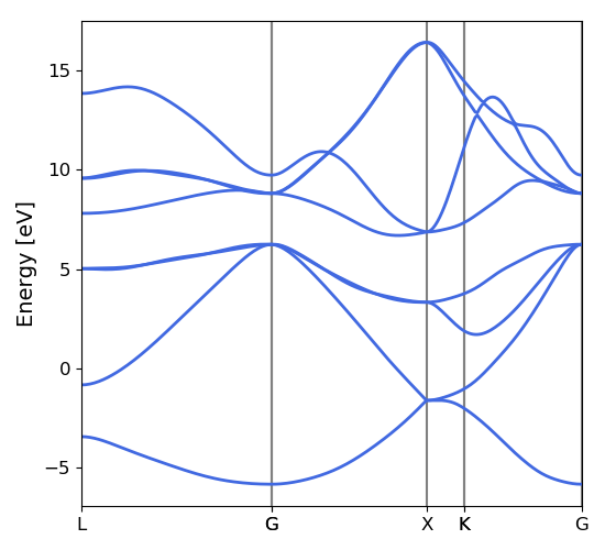
python bands.py electron_bands.json
# for the dos
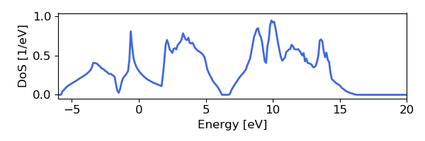
python dos.py electron_dos.json
This script will generate the following images, as below for the electron bands and DoS of silicon, found using Wannier interpolation (and a slightly more converged input calculation):
Convergence Checklist
As always, this is a demo calculation. However, it’s a very simple one, and there are only a few parameters which affect the end calculation.
The convergence of your electronic and phonon DFT calculations is of course, critical to this calculation (energy cutoff, k/q mesh, etc).
In particular, the electron Fourier interpolation can need many k-points to converge effectively. This is not a limitation of Phoebe – simply, Fourier interpolation requires many points to reach a high quality replication of the electronic structure.
You also should converge the DoS with respect to the kMesh/qMesh sampling of the Phoebe calculation.
Parallelization
The bands and DoS applications can take advantage of both OMP and MPI parallelization very effectively, and you should get an significant performance benefit from using either (or both) of these methods.